고정 헤더 영역
상세 컨텐츠
본문
로지시틱 회귀
우리가 직선으로 표현하지 못하는 경우 사용한다. 예로는 시험 점수 등이 있다.
선형 회귀와 유사한 방식으로 데이터를 모델링하지만, 주로 이진 분류 문제를 해결하는 데 사용
즉, 로지스틱 회귀는 주어진 입력 데이터가 특정 분류에 속할 확률을 예측하는 모델
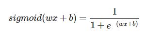
기본적으로 시그모이드(sigmoid)함수를 쓸수가 있다.
시그모이드 : 로지스틱 회귀에서는 출력값을 0과 1 사이의 확률로 제한하기 위해 시그모이드 함수(또는 로지스틱 함수)를 사용
확률예즉에 사용한다 했는데 예로는 이메일이 스팸인지 아닌지를 판단하는 모델을 만들 때, 모델은 주어진 이메일이 스팸일 확률을 출력 등이있다
추후에 한번 사용해봐야겠다.
import matplotlib.pyplot as plt
import pandas as pd
import numpy as np
from tensorflow import keras
from tensorflow.keras import layers
x = np.array([-50,-40,-35,-30,-25,-22, 10 ,25, 30, 45], dtype=np.float32)
y = np.array([0, 0, 0, 0, 0, 0, 1, 1, 1, 1], dtype=np.float32)

model = keras.Sequential([
    layers.Dense(units=1, input_shape=[1], activation='sigmoid')
])

init_w, init_b = model.get_weights()
print(init_w[0])
print(init_b

#### 초기화 값

sgd = keras.optimizers.SGD(learning_rate=0.01) # 경사하강법 0.1로 설정하고
model.compile(optimizer=sgd, loss='binary_crossentropy')

# 학습
history = model.fit(x, y, epochs=30)

# 학습된 w, b
w, b = model.get_weights()

print(f"\n\n\n학습된 w: {w}, b: {b}\n\n\n")

plt.scatter(x, y)

# k = np.linspace(-100, 100, 100)
z = 1 / (1 + np.exp(-(w[0] * x + b)))
plt.plot(x, z, color='red')
plt.title('trained Logistic Regression')
plt.show()

x_new = np.array(
    [-50,-10, 5, 10, 20],
    dtype=np.float32
)

y_new = np.round(model.predict(x_new), 3)

print(y_new)
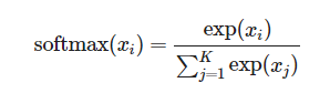
소프트맥스 회귀
다중 클래스 분류 문제에 사용되는 모델 ,지스틱 회귀가 이진 분류에 사용되는 반면, 소프트맥스 회귀는 세 개 이상의 클래스를 분류하는 데 적합
One-hot Encoding
범주형 레이블(예: '고양이', '개', '새')를 모델이 이해할 수 있는 형태로 변환합니다. 예를 들어, 3개의 클래스가 있다면 '고양이'는 [1, 0, 0], '개'는 [0, 1, 0], '새'는 [0, 0, 1]과 같이 표현됩니다.
소프트맥스 회귀 모델이 각 클래스에 대한 확률을 출력할 때, 실제 레이블과의 비교를 위해 one-hot encoding된 벡터가 사용됩니다.
소프트맥스 회귀는 교차 엔트로피 손실 함수를 사용하여 모델의 예측(확률 벡터)과 실제 레이블(one-hot encoded 벡터) 사이의 차이를 측정합니다.
이 과정에서 모델은 실제 레이블과 가장 가까운 확률 분포를 출력하도록 학습됩니다.
import matplotlib.pyplot as plt
import pandas as pd
import numpy as np
from tensorflow import keras
from tensorflow.keras import layers

x = np.array([
    [14, 5, 30],
    [16, 6, 45],
    [5, 5, 45],
    [20, 6, 60],
    [10, 7, 55],
    [13, 10, 50],
], dtype=np.float32)

y = np.array([
    [1,0,0], # 말티즈
    [0,1,0], # 푸들
    [0,0,1], # 치와와
    [1,0,0], # 말티즈
    [0,1,0], # 푸들
    [0,0,1], # 치와와
], dtype=np.float32)

model = keras.Sequential([
    layers.Dense(units=3, input_shape=[3], activation='softmax')
])

print(model.get_weights())


# 모델 컴파일 과정
sgd = keras.optimizers.SGD(learning_rate=0.01) # 경사하강법 learnig rate를 0.1로 설정하고
model.compile(optimizer=sgd, loss='categorical_crossentropy') # CCE를 비용함수로 설정

# 학습
history = model.fit(x, y, epochs=5)

# loss 시각화
plt.plot(history.history['loss'])
plt.title('Model Loss')
plt.xlabel('Epoch')
plt.ylabel('Loss')
plt.show()

# 새로운 데이터를 통한 label 예측
x_new = np.array([[12, 6, 35], [8, 5, 50]], dtype=np.float32)
y_pred = np.round(model.predict(x_new), 3)

# 모델이 예측한 label print
print(y_pred)
반응형
'코딩하는코알라 > AI' 카테고리의 다른 글
| 인공지능 개발 환경 이걸로끝(NVIDIA 드라이버 설치부터 CUDA까지) (0) | 2024.03.14 |
|---|---|
| 딥러닝 기본 용어 정의 (0) | 2024.02.05 |
| AI 학습을 위한 기본지식_선형회귀 (0) | 2024.02.01 |
| AI학습을 위한 기본적인 환경세팅 (0) | 2024.01.29 |
| Hugging Face의 Transformers 라이브러리_인코딩, 디코딩 (0) | 2024.01.21 |


